A HR image is generally considered a upscaled image of LR without losing any features or even better clarifing some features.
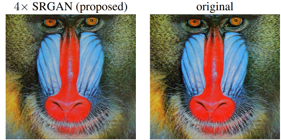
Here the left image is a SR image which is almost indistinguishable from the original HR image.
The highly challenging task of estimating a highresolution (HR) image from its low-resolution (LR) counterpart is referred to as super-resolution (SR).
This estimated image is called as super resolved (SR) image.
A HR image is generally considered a upscaled image of LR without losing any features or even better clarifing some features.
Here the left image is a SR image which is almost indistinguishable from the original HR image.
Before the SRGAN paper other methods such as interpolation, convulation network, etc. where used to generate a HR image out of LR image.
All these methods would calculate average values between the pixels to upscale the image and try to not loose the content of the image. This method of generating the HR image has produced decent result on the basis of our loss functions used previously such as MSE.
But as soon as the image is produced infront of a human they can clearly identify the mistakes in the generated image, thus this reliance on MSE as error method couldn't be accepted.
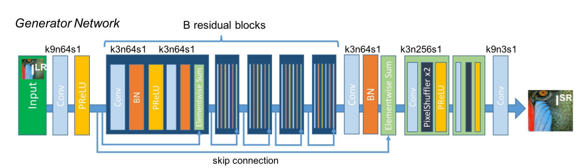
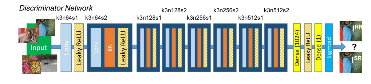
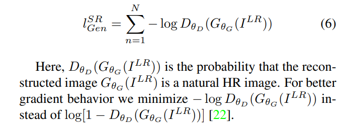
The SRGAN paper thus suggested to use a GAN network instead of a Convulational network model only thus dividing the loss into content loss and adverserial loss.
Like all GAN networks the architecture is divided into two parts:
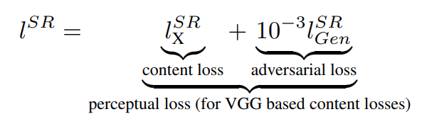
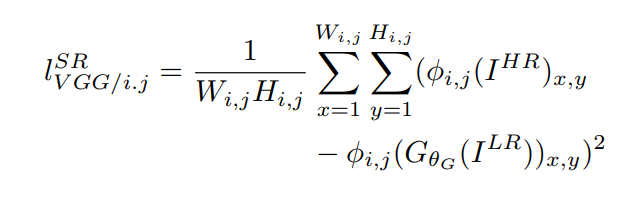
SRGAN use Preceptual loss which is a combination of content loss and adverserial loss.
The images for training were generated by download random image sets from internet and converting the images to HR(256 x 256) and LR (64 x 64) images of required sizes.
This was done by my short code I wrote below:
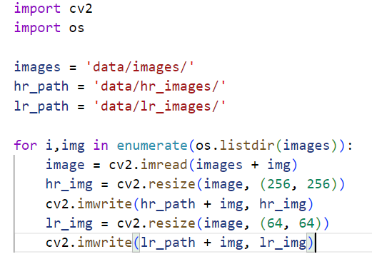
A total of around 1200 images were used out of which I did an 80/20 split for trainig and testing.
The model gnerated was only trained for about 30 epochs on limited data due to the unavailability of enough compute.
Even though of limited training the model showed enough improvement to demonstrate the possiblity of what can be achieved if enough compute is available.
Lets see the example of this image of a bike:
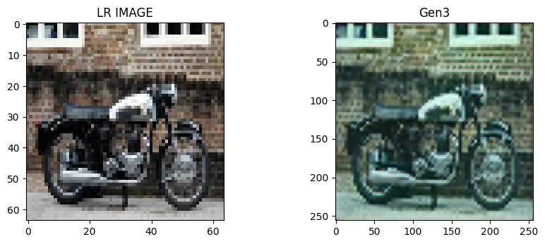
In the Gen3(Generator after 30 epochs) image we can clearly see the improvement over the edges of the bike than the LR image.
Here we can compare the models after 5 (Gen1), 15 (Gen2), 30(Gen3) epochs of training:
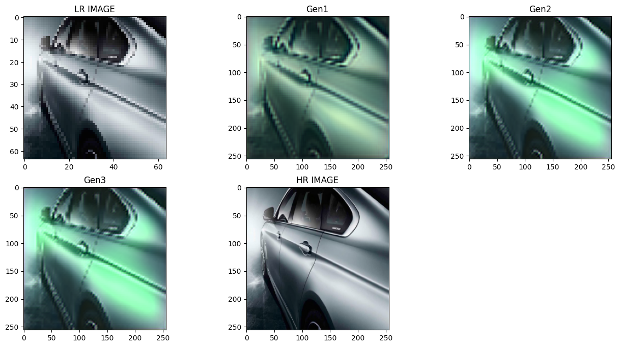
The Gen2 image of the car is way smoother than the Gen1 or the LR image, but there isn't any huge difference in Gen3. After epochs 15-20 there were only slight improvements over colors and textures.
From the two examples the main error of the model is seen to be color grading, bright white spots are green in generated images. The green spot increases in Gen2 but again decrease slightly on Gen3 which gives indication of not enough trainng.
This color grading problem may have arrised due to training of a saved model multiples times due to limited compute and the less data and train time given.
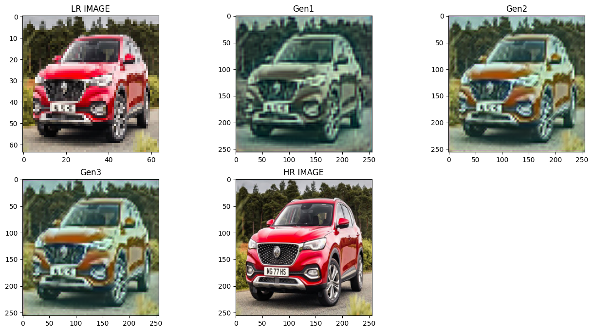
From this car test we can see the color improvement in Gen2 over Gen1. Thus given enough training it will fix the color grading.
Even though we couldn't get mind blowing results out of the model, we got enough improvement to see the possiblities.
This implementaion of a established paper was a fun learning exeperience.
I would recommend everyone to choose a paper and try to implement it in any capacity possible.