Vegetation Disease Detector
Introduction:
As Nepal is an agricultural focus country, the most common vegetation such as potatoes, tomatoes, Bell pepper, etc. are affected by several viruses and bacteria.
To combat this problem and detect some of the common diseases, viruses and bacteria we are using machine learning (neural network) and data analysis focused mainly on image processing.
Table of Content:
- Exploratory Data Analysis
- Visual interpretation of data
- Data split for train and validation
- Preprocessing images
- Model and layers definition
- Optimizers, Loss and metrics
- Results and Tests
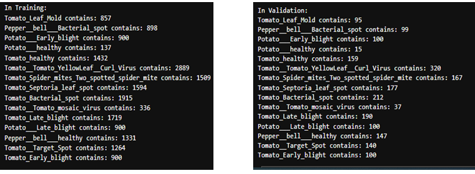
1. Exploratory Data Analysis:
The first step we take during any data science and machine learning project is exploring our data set.
The data set we use here is downloaded from here.
The main purpose of EDA is to help us better understand pattern the network will be able to find later on.

Here we can see we have data on 15 different conditions of vegetation from healthy to slight mold to even bacterial infection.
We also have a total of 20,638 images in total.
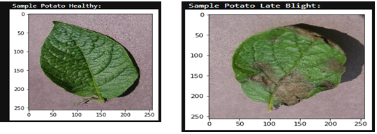
2. Visual Interpretation of Data:
We can observe for ourselves how much difference is there between and infected leave and a healthy one.
We take example of a tomato leaf, one is healthy and other is late blight.
3. Data split for training and validation:
Out of the 20,638 images we are using 90% of it for training and rest as validation data.
4. Preprocessing images:
Preprocessing refers to the process of preparing the data into form that is understood by the machine.
As everyone of know machines don’t understand images like we do they take it as a sequence of pixels each represented by a number.
Hence to easily convert these we use the tool provided by Keras API of Tensorflow called ImageDataGenerator.
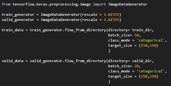
This tool makes all manual preprocessing tasks fast and easy.
5. Models and Layers:
For our sequential neural network we are using 3 2D Convolutional layers each of them followed by their own 2D Max Polling layer.
Then a 25% dropout layer feeding into a flattening layer.
After the flattening layer the main 1024 neural Dense layer is located which feeds into our 15 neural output layer.
All these Convolutional layers and Dense have relu as their activation function where as our output layer has a softmax activation function.
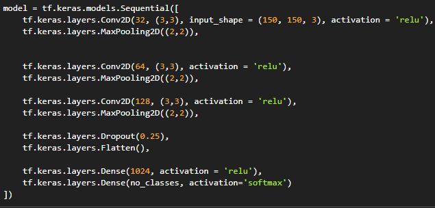
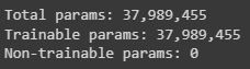
We have a total of 37,989,455 parameters in our mode out of which all are trainable parameters.
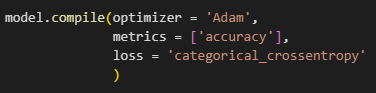
6. Optimizers, Loss and Metrics:
We are evaluating the performance of our model based on the accuracy metric.
The optimizer used in the model is Adam and categorical-crossentropy as our loss function from Keras Api of Tensorflow.
7. Results:
After training the model on our training set we got a training accuracy of 98% and 0.0408 loss.
Similarly on the validation set we got a final accuracy of 92% and 0.3488 loss.
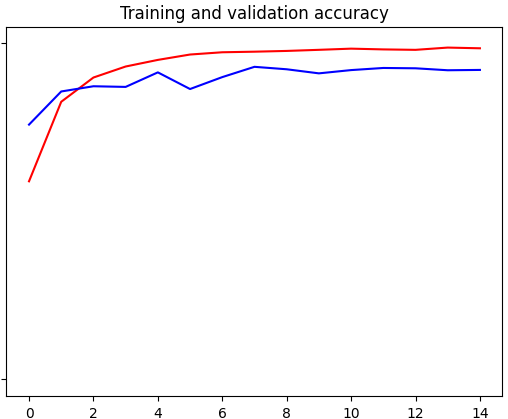
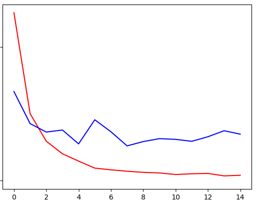
Red line - Training accuracy and Loss
Blue line - validation accuracy and Loss